single
Rand Index
Свайпніть щоб показати меню
Well, you may notice, that dendrograms look a bit different. Using a single linkage it's hard to define 4 clusters because the heights on the right side are too small. But complete linkage makes us think that 4 clusters are possible. Okay, we can experiment and compare the dendrograms, but what about the clustering results? Can we compare them?
The answer is yes, we can. The two clustering results can be compared by using Rand Index, which compares predicted labels across two models, and returns the number between 0 and 1. 1.0 stands for a perfect match, while 0.0 stands for an absolute lack of similarities between predicted labels.
In Python, you can access the rand index by using the rand_score() function from the sklearn.metrics library. This function receives only two parameters: predicted labels by two models. It's obvious that both lists/arrays must be the same size.
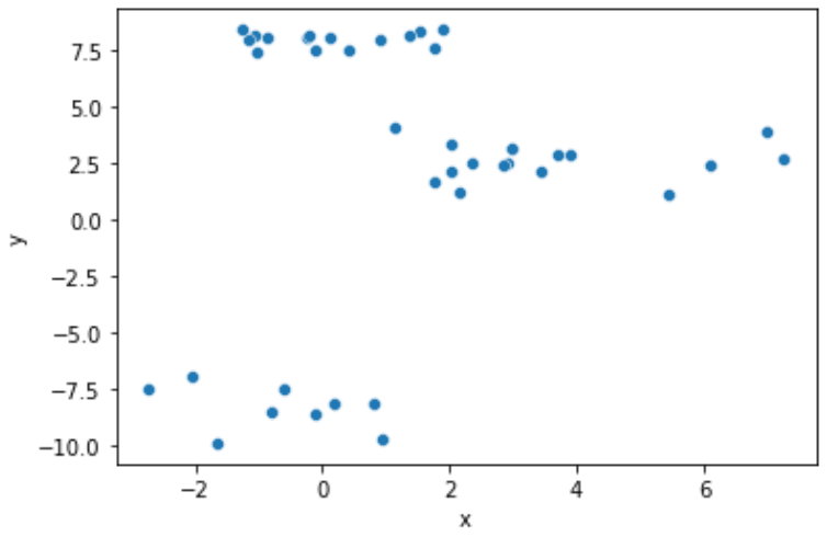
For example, we can compare the result of clustering well-clustered data (scatter plot is below) while using two different linkages: 'single' and 'ward'. To set linkage while clustering you need to set the linkage = '...' parameter within AgglomerativeClustering() function.
1234567891011121314151617181920# Import the libraries import pandas as pd import matplotlib.pyplot as plt from sklearn.metrics import rand_score from sklearn.cluster import AgglomerativeClustering # Read the data data = pd.read_csv('https://codefinity-content-media.s3.eu-west-1.amazonaws.com/138ab9ad-aa37-4310-873f-0f62abafb038/model_data1.csv') # Creating the models model_single = AgglomerativeClustering(n_clusters = 3, linkage = 'single') model_ward = AgglomerativeClustering(n_clusters = 3, linkage = 'ward') # Fitting and predicting the labels labels_single = model_single.fit_predict(data) labels_ward = model_ward.fit_predict(data) # Compute the Rand index rand_index = rand_score(labels_single, labels_ward) print(f"The rand index for single and ward linkages models is {rand_index}")
This code will output the following message:
The rand index for single and ward linkages models is 1.0
This means that both linkages will lead us to identical clustering results. This is kinda obvious since the points are divided into 3 clear clusters.
But what about the data we used in the previous chapters? Let's find out how similar will be models with different linkages used.
Проведіть, щоб почати кодувати
Let's figure out how close will be the results for the data from the last 2 previous chapters if we would like to split them into 4 clusters. The scatter plot is below.
Follow the next steps:
- Import
rand_scoreandAgglomerativeClusteringfromsklearn.metricsandsklearn.clusterrespectively. - Create two
AgglomerativeClusteringobjects:
-
model_singlewith 4 clusters and'single'linkage. -
model_completewith 4 clusters and'complete'linkage.- Fit the data to model and predict the labels:
-
labels_singlefor the labels predicted by themodel_singlemodel. -
labels_completefor the labels predicted by themodel_completemodel.- Compute the rand score using
labels_singleandlabels_complete.
- Compute the rand score using
Рішення
Дякуємо за ваш відгук!
single
Запитати АІ
Запитати АІ

Запитайте про що завгодно або спробуйте одне із запропонованих запитань, щоб почати наш чат
