Seção 3. Capítulo 8
single
How Similar are the Results?
Deslize para mostrar o menu
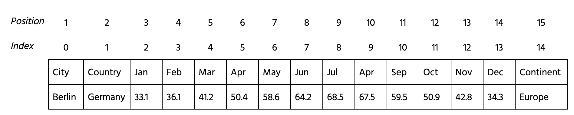
Well done! Let's look at the last line charts you built in the previous chapter.
As you can see, only the ward linkage could catch the 'downward up to July' trend. Both results are different. But let's find out how different they are using the rand index.
Tarefa
Deslize para começar a programar
Compute the rand index to compare the results of using complete and ward linkages. Follow the next steps:
- Import functions needed:
rand_scorefromsklearn.metrics.AgglomerativeClusteringfromsklearn.cluster.
- Create two models
model_completeandmodel_wardperforming a hierarchical clustering with 4 clusters both and'complete'and'ward'linkages respectively. - Fit the 3-14 columns of
datato models and predict the labels. Save the labels formodel_completewithinlabels_completeand formodel_wardwithinlabels_ward. - Compute the rand index using
labels_completeandlabels_ward.
Solução
Tudo estava claro?
Obrigado pelo seu feedback!
Seção 3. Capítulo 8
single
Pergunte à IA
Pergunte à IA

Pergunte o que quiser ou experimente uma das perguntas sugeridas para iniciar nosso bate-papo
