Using Slicers and Timelines
Scorri per mostrare il menu
In professional reporting, users rarely want static tables. Managers want to filter data quickly, compare scenarios, and explore trends without rebuilding Pivot Tables.
Slicers and Timelines provide interactive controls that allow dynamic filtering without modifying the Pivot structure.
Why This Matters in Real Reporting
Use slicers to:
- Filter reports by Region during meetings;
- Compare performance across categories instantly;
- Switch between time periods;
- Create clean interactive dashboards.
Instead of opening dropdown menus, slicers provide visual buttons. Timelines provide visual control over date filtering.
What Is a Slicer?
A Slicer is a visual filtering panel connected to a Pivot Table. It allows you to: click one or multiple items, instantly filter the Pivot, clear filters easily, see active filters visually.
How to Insert a Slicer
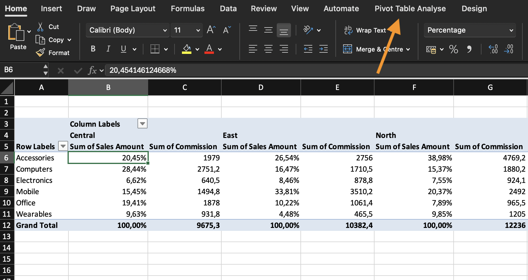
- Click inside the Pivot Table;
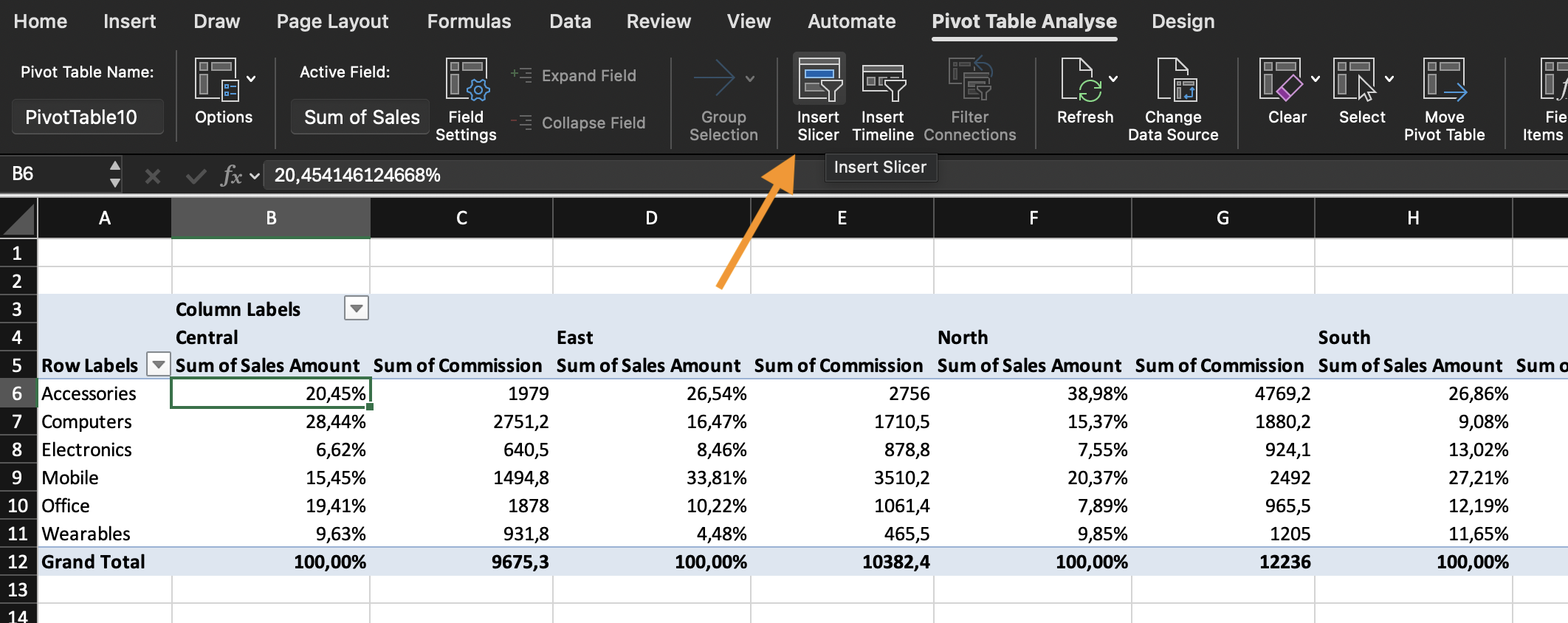
- Go to PivotTable Analyze tab;
- Click Insert Slicer;
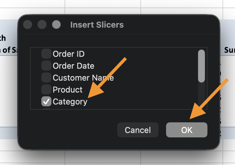
- Select one or more fields (e.g., Category, Region);
- Click OK.
A visual filter panel appears. You can: resize it, change column layout, apply multiple selections.


What Is a Timeline?
A Timeline is a specialized slicer for date fields. It allows filtering by: year, quarter, month, day.
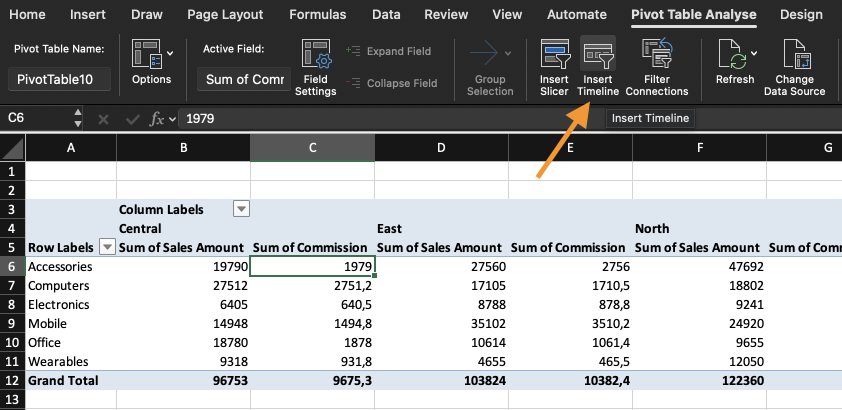
How to Insert a Timeline
- Click inside the Pivot Table;
- Go to PivotTable Analyze;
- Click Insert Timeline;
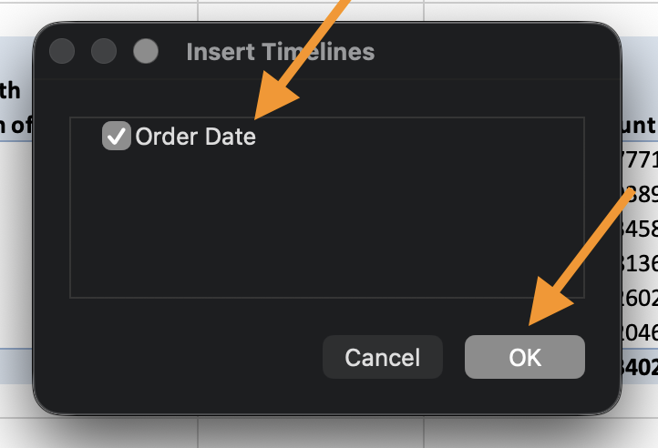
- Select a Date field;
- Click OK.
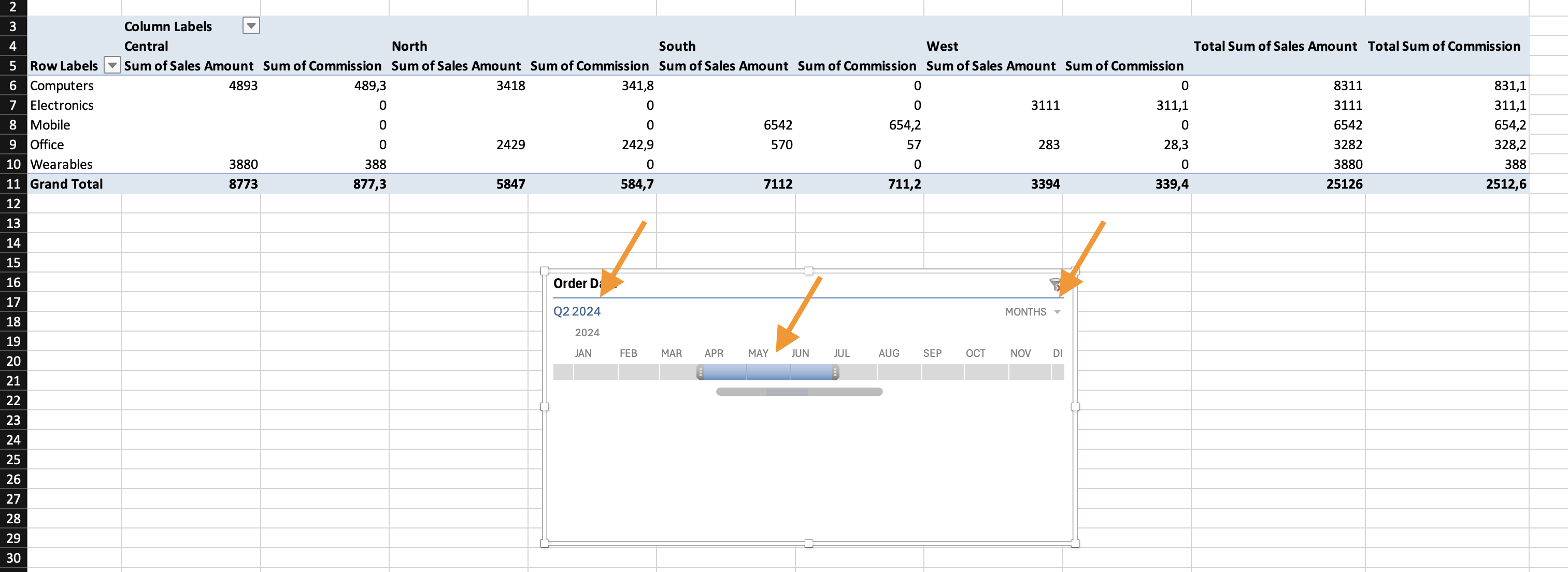
You can: switch between Years / Quarters / Months, drag the slider to filter periods, and select multiple time ranges.
Task
- Create Pivot Table #1:
- Rows: Category;
- Values: Sum of Revenue.
- Create Pivot Table #2:
- Rows: Region;
- Values: Sum of Revenue.
- Insert:
- Slicer for Category;
- Slicer for Region;
- Timeline for Date.
- After creating both Pivot Tables and connecting all slicers, apply the following filters:
- Select: Appliances, Electronics, Home Decor, Sports;
- Select: East, South, West;
- Filter the Date field to show: Quarter 2 only.
When you insert a slicer, it connects only to the Pivot Table that was active at the time of insertion.
If you have multiple Pivot Tables and want them to respond to the same slicer, you must connect them manually.
How to Connect a Slicer to Multiple Pivot Tables
- Click on the slicer;
- Go to the Slicer tab (or Slicer Options);
- Click Report Connections (In some Excel versions this is called PivotTable Connections);
- A dialog box appears showing all Pivot Tables based on the same data source;
- Check the boxes for the Pivot Tables you want to connect;
- Click OK.
Now the slicer controls all selected Pivot Tables simultaneously.
All Pivot Tables must be built from the same data source.
Grazie per i tuoi commenti!
Chieda ad AI
Chieda ad AI

Chieda pure quello che desidera o provi una delle domande suggerite per iniziare la nostra conversazione
Using Slicers and Timelines
In professional reporting, users rarely want static tables. Managers want to filter data quickly, compare scenarios, and explore trends without rebuilding Pivot Tables.
Slicers and Timelines provide interactive controls that allow dynamic filtering without modifying the Pivot structure.
Why This Matters in Real Reporting
Use slicers to:
- Filter reports by Region during meetings;
- Compare performance across categories instantly;
- Switch between time periods;
- Create clean interactive dashboards.
Instead of opening dropdown menus, slicers provide visual buttons. Timelines provide visual control over date filtering.
What Is a Slicer?
A Slicer is a visual filtering panel connected to a Pivot Table. It allows you to: click one or multiple items, instantly filter the Pivot, clear filters easily, see active filters visually.
How to Insert a Slicer
- Click inside the Pivot Table;
- Go to PivotTable Analyze tab;
- Click Insert Slicer;
- Select one or more fields (e.g., Category, Region);
- Click OK.
A visual filter panel appears. You can: resize it, change column layout, apply multiple selections.
What Is a Timeline?
A Timeline is a specialized slicer for date fields. It allows filtering by: year, quarter, month, day.
How to Insert a Timeline
- Click inside the Pivot Table;
- Go to PivotTable Analyze;
- Click Insert Timeline;
- Select a Date field;
- Click OK.
You can: switch between Years / Quarters / Months, drag the slider to filter periods, and select multiple time ranges.
Task
- Create Pivot Table #1:
- Rows: Category;
- Values: Sum of Revenue.
- Create Pivot Table #2:
- Rows: Region;
- Values: Sum of Revenue.
- Insert:
- Slicer for Category;
- Slicer for Region;
- Timeline for Date.
- After creating both Pivot Tables and connecting all slicers, apply the following filters:
- Select: Appliances, Electronics, Home Decor, Sports;
- Select: East, South, West;
- Filter the Date field to show: Quarter 2 only.
When you insert a slicer, it connects only to the Pivot Table that was active at the time of insertion.
If you have multiple Pivot Tables and want them to respond to the same slicer, you must connect them manually.
How to Connect a Slicer to Multiple Pivot Tables
- Click on the slicer;
- Go to the Slicer tab (or Slicer Options);
- Click Report Connections (In some Excel versions this is called PivotTable Connections);
- A dialog box appears showing all Pivot Tables based on the same data source;
- Check the boxes for the Pivot Tables you want to connect;
- Click OK.
Now the slicer controls all selected Pivot Tables simultaneously.
All Pivot Tables must be built from the same data source.
Grazie per i tuoi commenti!
