Desafío: Construcción de una CNN
Desliza para mostrar el menú
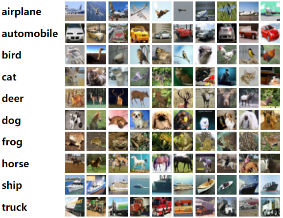
Las redes neuronales convolucionales (CNN) se utilizan ampliamente en la clasificación de imágenes debido a su capacidad para extraer características jerárquicas. En esta tarea, se implementará y entrenará una CNN similar a VGG utilizando TensorFlow y Keras en el conjunto de datos CIFAR-10. El conjunto de datos consta de 60,000 imágenes (32×32×3) pertenecientes a 10 clases diferentes, incluyendo aviones, automóviles, aves, gatos y más.
Este proyecto guiará a través de la carga del conjunto de datos, el preprocesamiento de las imágenes, la definición del modelo CNN, su entrenamiento y la evaluación de su rendimiento.
1. Preprocesamiento de datos para CNN
Antes de entrenar una CNN, el preprocesamiento de los datos es un paso crucial para asegurar un mejor rendimiento y una convergencia más rápida. Los métodos de preprocesamiento comunes incluyen:
-
Normalización: este método consiste en escalar los valores de los píxeles de las imágenes de un rango entre 0 y 255 a un rango entre 0 y 1. A menudo se implementa como
x_train / 255.0, x_test / 255.0; -
Codificación one-hot: las etiquetas suelen convertirse en vectores codificados one-hot para tareas de clasificación. Esto se realiza típicamente utilizando la función
keras.utils.to_categorical, que transforma etiquetas enteras (por ejemplo, 0, 1, 2, etc.) en un vector codificado one-hot, como[1, 0, 0, 0]para un problema de clasificación de 4 clases.
2. Construcción de la arquitectura CNN
Una arquitectura CNN está compuesta por varias capas que realizan diferentes tareas para extraer características y hacer predicciones. Puedes implementar las capas clave de una CNN mediante:
Capa convolucional (Conv2D)
keras.layers.Conv2D(filters, kernel_size, activation='relu', padding='same', input_shape=(height, width, channels))
El parámetro input_shape solo debe especificarse en la capa de entrada.
Capa de agrupamiento (MaxPooling2D)
keras.layers.MaxPooling2D(pool_size=(2, 2))
Capa Flatten
keras.layers.Flatten()
Capa Dense
layers.Dense(units=512, activation='relu')
layers.Dense(10, activation='softmax')
La capa densa final normalmente tiene un número de unidades igual al número de clases y utiliza una función de activación softmax para generar una distribución de probabilidad entre las clases.
3. Compilación del modelo
Después de definir la arquitectura, es necesario compilar el modelo. Este paso implica especificar la función de pérdida, el optimizador y las métricas que guiarán al modelo durante el entrenamiento. Los siguientes métodos son comúnmente utilizados en las CNN:
Optimizador (Adam)
El optimizador ajusta los pesos del modelo para minimizar la función de pérdida. El optimizador Adam es popular debido a su eficiencia y capacidad para adaptar la tasa de aprendizaje durante el entrenamiento.
keras.optimizers.Adam()
Función de pérdida (Categorical Crossentropy)
Para la clasificación multiclase, normalmente se utiliza la función de pérdida categorical crossentropy. Esto se puede implementar como:
keras.losses.CategoricalCrossentropy()
Métricas
El rendimiento del modelo se monitorea utilizando métricas para tareas de clasificación, como precisión, exactitud, recall, etc. Estas se pueden definir como:
metrics = [
    keras.metrics.Accuracy(),
    keras.metrics.Precision(),
    keras.metrics.Recall()
]
Compilar
model.compile(optimizer='adam',
              loss='categorical_crossentropy', # Or keras.losses.CategoricalCrossentropy()
              metrics=metrics)
4. Entrenamiento del modelo
El entrenamiento de una CNN consiste en alimentar los datos de entrada a la red, calcular la función de pérdida y actualizar los pesos mediante retropropagación. El proceso de entrenamiento se controla mediante los siguientes métodos clave:
- Ajuste del modelo: el método
fit()se utiliza para entrenar el modelo. Este método recibe los datos de entrenamiento, el número de épocas y el tamaño de lote. También incluye una división opcional de validación para evaluar el rendimiento del modelo en datos no vistos durante el entrenamiento:
history = model.fit(x_train, y_train, epochs=10, batch_size=32, validation_split=0.2)
- Tamaño de lote y épocas: el tamaño de lote determina el número de muestras procesadas antes de actualizar los pesos del modelo, y el número de épocas se refiere a cuántas veces se pasa el conjunto de datos completo por el modelo.
5. Evaluación
Informe de Clasificación
sklearn.metrics.classification_report() compara los valores verdaderos y predichos del conjunto de prueba. Incluye precisión, recall y puntuación F1 para cada clase. Sin embargo, los métodos necesitan solo las etiquetas de clase, así que no olvides convertirlas de nuevo desde los vectores ([0,0,1,0] -> 2):
y_pred = model.predict(x_test)
y_pred_classes = np.argmax(y_pred,axis = 1)
y_test_classes = np.argmax(y_test, axis = 1)

report = classification_report(y_test_classes, y_pred_classes, target_names=class_names)
print(report)
Evaluar
Una vez que el modelo está entrenado, se evalúa en el conjunto de prueba para medir su capacidad de generalización. La evaluación proporciona métricas, que se mencionaron en el método .compile(). La evaluación se realiza usando .evaluate():
results = model.evaluate(x_test, y_test, verbose=2, return_dict=True)
Matriz de Confusión
Para obtener más información sobre el rendimiento del modelo, se puede visualizar la matriz de confusión, que muestra las predicciones verdaderos positivos, falsos positivos, verdaderos negativos y falsos negativos para cada clase. La matriz de confusión se puede calcular usando TensorFlow:
confusion_mtx = tf.math.confusion_matrix(y_test_classes, y_pred_classes)
Esta matriz puede visualizarse utilizando mapas de calor para observar el desempeño del modelo en cada clase:
plt.figure(figsize=(12, 9))
c = sns.heatmap(confusion_mtx, annot=True, fmt='g')
c.set(xticklabels=class_names, yticklabels=class_names)

plt.show()
Tarea
1. Cargar y preprocesar el conjunto de datos
- Importar el conjunto de datos CIFAR-10 desde Keras;
- Normalizar los valores de los píxeles al rango
[0,1]para una mejor convergencia; - Convertir las etiquetas de clase al formato
one-hot encodedpara clasificación categórica.
2. Definir el modelo CNN
Implementación de una arquitectura CNN tipo VGG con las siguientes capas clave:

Capas convolucionales:
- Tamaño del kernel:
3×3; - Función de activación:
ReLU; - Relleno:
'same'.
Capas de pooling:
- Tipo de pooling:
max pooling; - Tamaño de pooling:
2×2.
Capas de dropout (Prevención de sobreajuste deshabilitando aleatoriamente neuronas):
- Tasa de dropout:
25%.
Capa de flatten - conversión de mapas de características 2D en un vector 1D para clasificación.
Capas completamente conectadas - capas densas para la clasificación final, con una capa de salida relu o softmax.
Compilar el modelo usando:
Adam optimizer(aprendizaje eficiente);- Función de pérdida
Categorical cross-entropy(para clasificación multiclase); - Métrica de
Accuracy metricpara medir el rendimiento (las clases están balanceadas, y puedes agregar otras métricas si lo deseas).
3. Entrenar el modelo
- Especificar los parámetros
epochsybatch_sizepara el entrenamiento (por ejemplo,epochs=20, batch_size=64); - Especificar el parámetro
validation_splitpara definir el porcentaje de datos de entrenamiento que se utilizarán como validación para monitorear el rendimiento del modelo en imágenes no vistas; - Guardar el historial de entrenamiento para visualizar tendencias de precisión y pérdida.
4. Evaluar y visualizar resultados
- Probar el modelo en los datos de prueba de CIFAR-10 e imprimir la precisión;
- Graficar pérdida de entrenamiento vs. pérdida de validación para verificar sobreajuste;
- Graficar precisión de entrenamiento vs. precisión de validación para asegurar la progresión del aprendizaje.
¡Gracias por tus comentarios!
Pregunte a AI
Pregunte a AI

Pregunte lo que quiera o pruebe una de las preguntas sugeridas para comenzar nuestra charla
Desafío: Construcción de una CNN
Las redes neuronales convolucionales (CNN) se utilizan ampliamente en la clasificación de imágenes debido a su capacidad para extraer características jerárquicas. En esta tarea, se implementará y entrenará una CNN similar a VGG utilizando TensorFlow y Keras en el conjunto de datos CIFAR-10. El conjunto de datos consta de 60,000 imágenes (32×32×3) pertenecientes a 10 clases diferentes, incluyendo aviones, automóviles, aves, gatos y más.
Este proyecto guiará a través de la carga del conjunto de datos, el preprocesamiento de las imágenes, la definición del modelo CNN, su entrenamiento y la evaluación de su rendimiento.
1. Preprocesamiento de datos para CNN
Antes de entrenar una CNN, el preprocesamiento de los datos es un paso crucial para asegurar un mejor rendimiento y una convergencia más rápida. Los métodos de preprocesamiento comunes incluyen:
-
Normalización: este método consiste en escalar los valores de los píxeles de las imágenes de un rango entre 0 y 255 a un rango entre 0 y 1. A menudo se implementa como
x_train / 255.0, x_test / 255.0; -
Codificación one-hot: las etiquetas suelen convertirse en vectores codificados one-hot para tareas de clasificación. Esto se realiza típicamente utilizando la función
keras.utils.to_categorical, que transforma etiquetas enteras (por ejemplo, 0, 1, 2, etc.) en un vector codificado one-hot, como[1, 0, 0, 0]para un problema de clasificación de 4 clases.
2. Construcción de la arquitectura CNN
Una arquitectura CNN está compuesta por varias capas que realizan diferentes tareas para extraer características y hacer predicciones. Puedes implementar las capas clave de una CNN mediante:
Capa convolucional (Conv2D)
keras.layers.Conv2D(filters, kernel_size, activation='relu', padding='same', input_shape=(height, width, channels))
El parámetro input_shape solo debe especificarse en la capa de entrada.
Capa de agrupamiento (MaxPooling2D)
keras.layers.MaxPooling2D(pool_size=(2, 2))
Capa Flatten
keras.layers.Flatten()
Capa Dense
layers.Dense(units=512, activation='relu')
layers.Dense(10, activation='softmax')
La capa densa final normalmente tiene un número de unidades igual al número de clases y utiliza una función de activación softmax para generar una distribución de probabilidad entre las clases.
3. Compilación del modelo
Después de definir la arquitectura, es necesario compilar el modelo. Este paso implica especificar la función de pérdida, el optimizador y las métricas que guiarán al modelo durante el entrenamiento. Los siguientes métodos son comúnmente utilizados en las CNN:
Optimizador (Adam)
El optimizador ajusta los pesos del modelo para minimizar la función de pérdida. El optimizador Adam es popular debido a su eficiencia y capacidad para adaptar la tasa de aprendizaje durante el entrenamiento.
keras.optimizers.Adam()
Función de pérdida (Categorical Crossentropy)
Para la clasificación multiclase, normalmente se utiliza la función de pérdida categorical crossentropy. Esto se puede implementar como:
keras.losses.CategoricalCrossentropy()
Métricas
El rendimiento del modelo se monitorea utilizando métricas para tareas de clasificación, como precisión, exactitud, recall, etc. Estas se pueden definir como:
metrics = [
    keras.metrics.Accuracy(),
    keras.metrics.Precision(),
    keras.metrics.Recall()
]
Compilar
model.compile(optimizer='adam',
              loss='categorical_crossentropy', # Or keras.losses.CategoricalCrossentropy()
              metrics=metrics)
4. Entrenamiento del modelo
El entrenamiento de una CNN consiste en alimentar los datos de entrada a la red, calcular la función de pérdida y actualizar los pesos mediante retropropagación. El proceso de entrenamiento se controla mediante los siguientes métodos clave:
- Ajuste del modelo: el método
fit()se utiliza para entrenar el modelo. Este método recibe los datos de entrenamiento, el número de épocas y el tamaño de lote. También incluye una división opcional de validación para evaluar el rendimiento del modelo en datos no vistos durante el entrenamiento:
history = model.fit(x_train, y_train, epochs=10, batch_size=32, validation_split=0.2)
- Tamaño de lote y épocas: el tamaño de lote determina el número de muestras procesadas antes de actualizar los pesos del modelo, y el número de épocas se refiere a cuántas veces se pasa el conjunto de datos completo por el modelo.
5. Evaluación
Informe de Clasificación
sklearn.metrics.classification_report() compara los valores verdaderos y predichos del conjunto de prueba. Incluye precisión, recall y puntuación F1 para cada clase. Sin embargo, los métodos necesitan solo las etiquetas de clase, así que no olvides convertirlas de nuevo desde los vectores ([0,0,1,0] -> 2):
y_pred = model.predict(x_test)
y_pred_classes = np.argmax(y_pred,axis = 1)
y_test_classes = np.argmax(y_test, axis = 1)

report = classification_report(y_test_classes, y_pred_classes, target_names=class_names)
print(report)
Evaluar
Una vez que el modelo está entrenado, se evalúa en el conjunto de prueba para medir su capacidad de generalización. La evaluación proporciona métricas, que se mencionaron en el método .compile(). La evaluación se realiza usando .evaluate():
results = model.evaluate(x_test, y_test, verbose=2, return_dict=True)
Matriz de Confusión
Para obtener más información sobre el rendimiento del modelo, se puede visualizar la matriz de confusión, que muestra las predicciones verdaderos positivos, falsos positivos, verdaderos negativos y falsos negativos para cada clase. La matriz de confusión se puede calcular usando TensorFlow:
confusion_mtx = tf.math.confusion_matrix(y_test_classes, y_pred_classes)
Esta matriz puede visualizarse utilizando mapas de calor para observar el desempeño del modelo en cada clase:
plt.figure(figsize=(12, 9))
c = sns.heatmap(confusion_mtx, annot=True, fmt='g')
c.set(xticklabels=class_names, yticklabels=class_names)

plt.show()
Tarea
1. Cargar y preprocesar el conjunto de datos
- Importar el conjunto de datos CIFAR-10 desde Keras;
- Normalizar los valores de los píxeles al rango
[0,1]para una mejor convergencia; - Convertir las etiquetas de clase al formato
one-hot encodedpara clasificación categórica.
2. Definir el modelo CNN
Implementación de una arquitectura CNN tipo VGG con las siguientes capas clave:
Capas convolucionales:
- Tamaño del kernel:
3×3; - Función de activación:
ReLU; - Relleno:
'same'.
Capas de pooling:
- Tipo de pooling:
max pooling; - Tamaño de pooling:
2×2.
Capas de dropout (Prevención de sobreajuste deshabilitando aleatoriamente neuronas):
- Tasa de dropout:
25%.
Capa de flatten - conversión de mapas de características 2D en un vector 1D para clasificación.
Capas completamente conectadas - capas densas para la clasificación final, con una capa de salida relu o softmax.
Compilar el modelo usando:
Adam optimizer(aprendizaje eficiente);- Función de pérdida
Categorical cross-entropy(para clasificación multiclase); - Métrica de
Accuracy metricpara medir el rendimiento (las clases están balanceadas, y puedes agregar otras métricas si lo deseas).
3. Entrenar el modelo
- Especificar los parámetros
epochsybatch_sizepara el entrenamiento (por ejemplo,epochs=20, batch_size=64); - Especificar el parámetro
validation_splitpara definir el porcentaje de datos de entrenamiento que se utilizarán como validación para monitorear el rendimiento del modelo en imágenes no vistas; - Guardar el historial de entrenamiento para visualizar tendencias de precisión y pérdida.
4. Evaluar y visualizar resultados
- Probar el modelo en los datos de prueba de CIFAR-10 e imprimir la precisión;
- Graficar pérdida de entrenamiento vs. pérdida de validación para verificar sobreajuste;
- Graficar precisión de entrenamiento vs. precisión de validación para asegurar la progresión del aprendizaje.
¡Gracias por tus comentarios!
