Dynamic Charts with Formulas
Swipe to show menu
A dynamic chart range is a data range that changes automatically based on a condition or selection. Instead of building a chart from a fixed range, you build it from a formula-driven range. When the formula result changes, the chart updates. The chart itself is not dynamic. The data source is.
How It Works
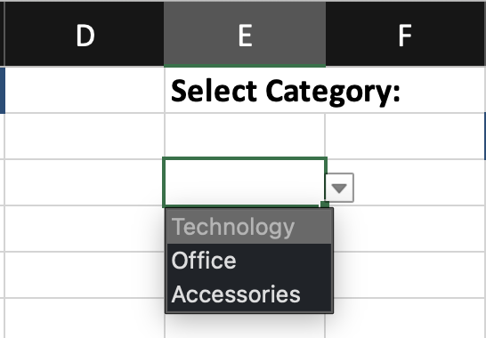
- A user selects a value from a dropdown;
- A formula returns only the matching rows;
- The chart is built from that formula output;
- When the selection changes, the formula output changes;
- The chart updates automatically.
The key idea: the chart depends on a formula range, not the full dataset.
Creating the Dynamic Range
Assume:
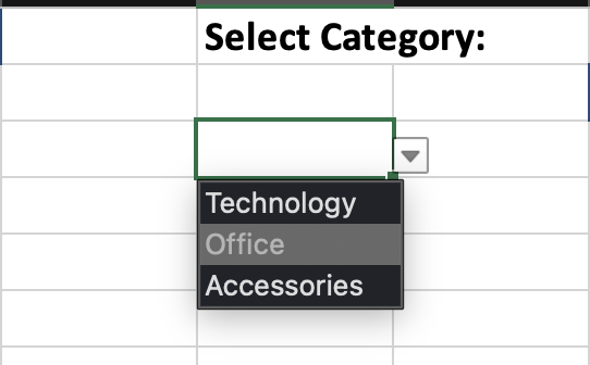
Step 1: Create a Dropdown
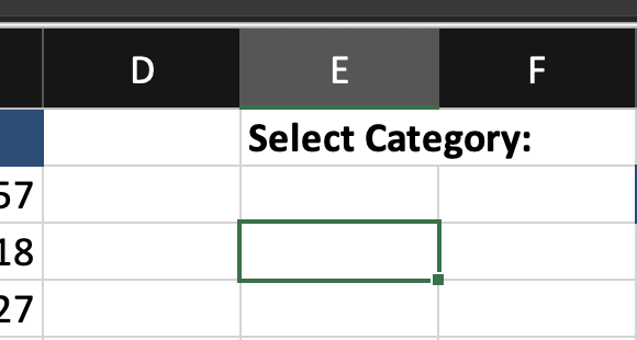
- Select an empty cell;
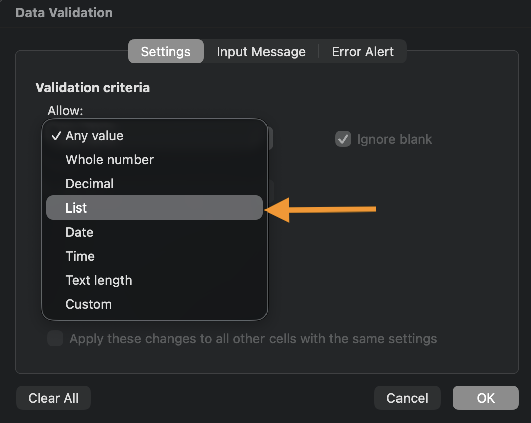
- Go to Data → Data Validation;
- Choose List;
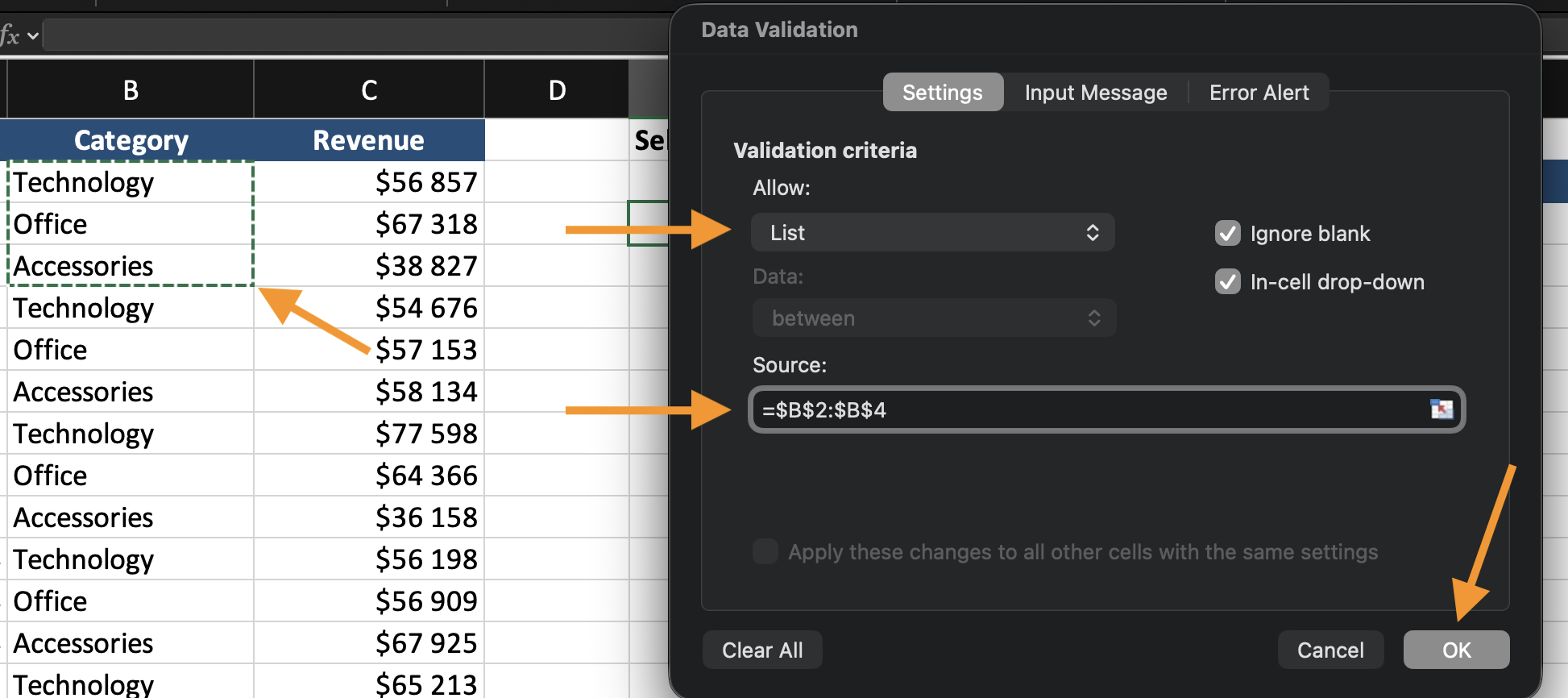
- Select the category range.

Step 2: Create the Formula Output
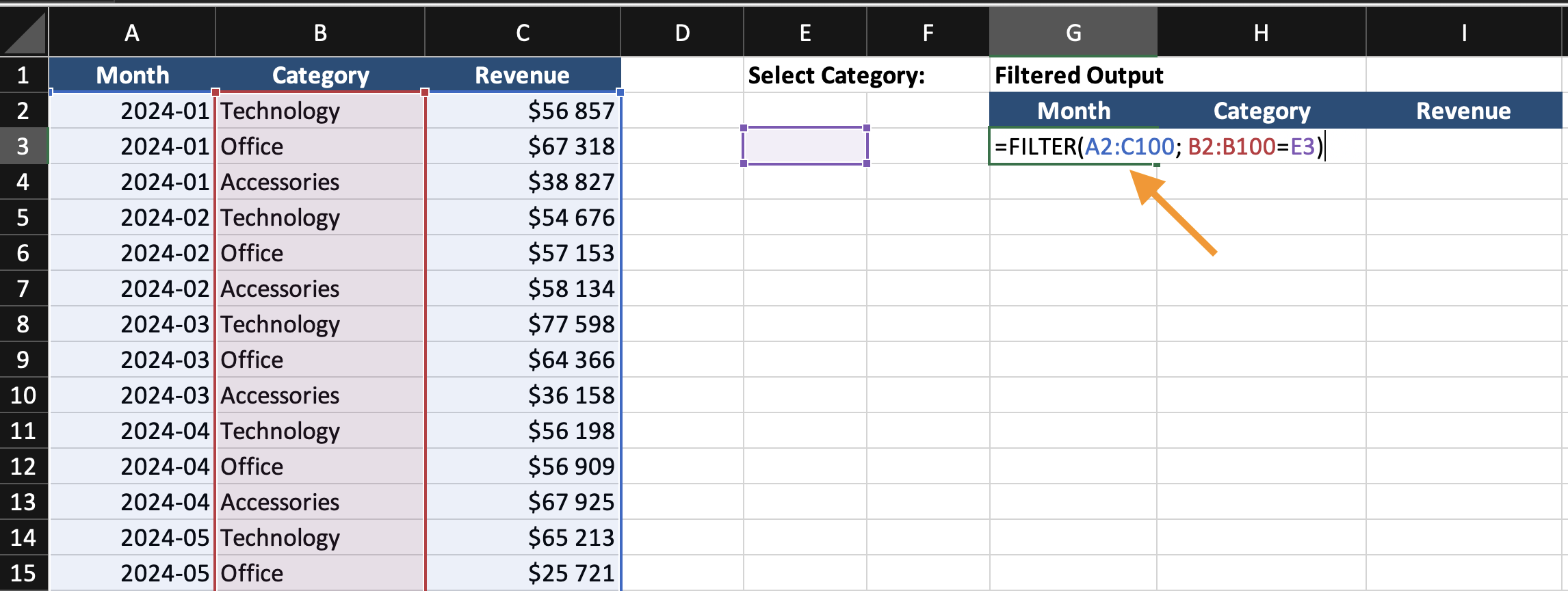
In a new area, enter: =FILTER(A2:C100; B2:B100=E2)
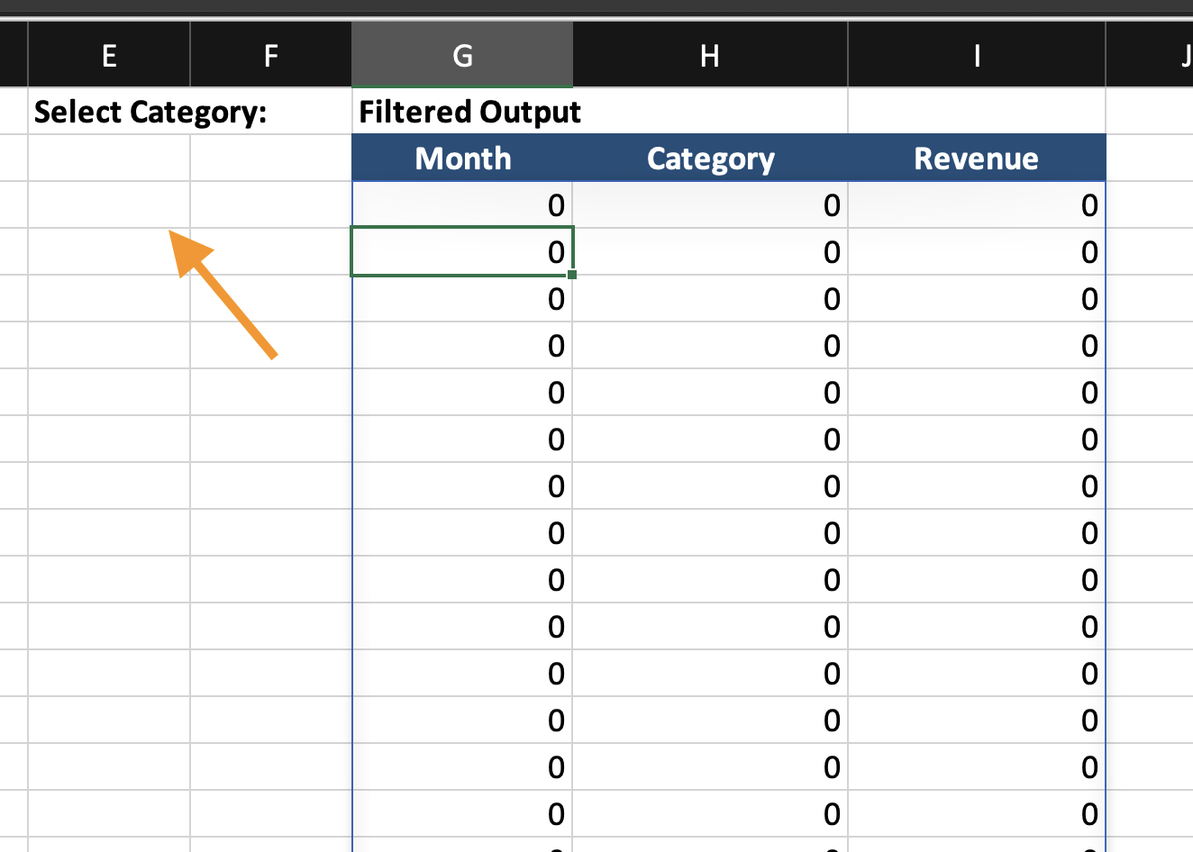
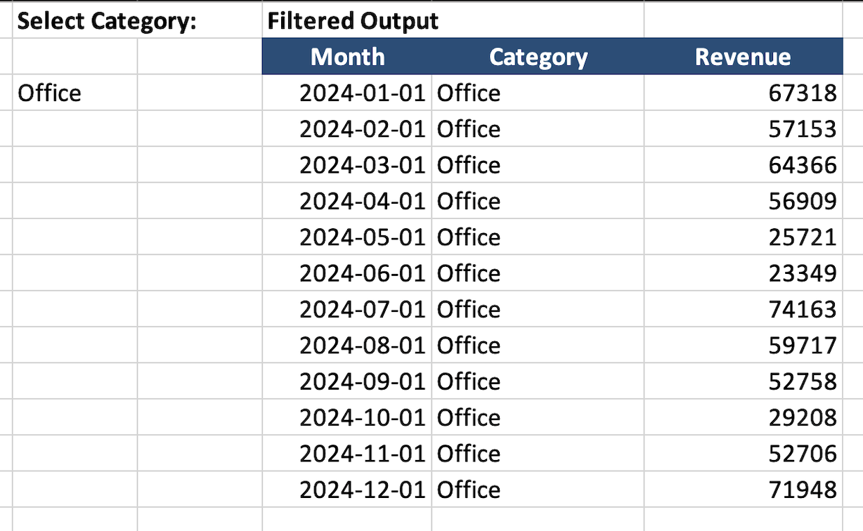
This creates a dynamic output table.
Step 3: Build the Chart
Insert a chart using the filtered output, not the original data. Now the chart updates when the dropdown changes.
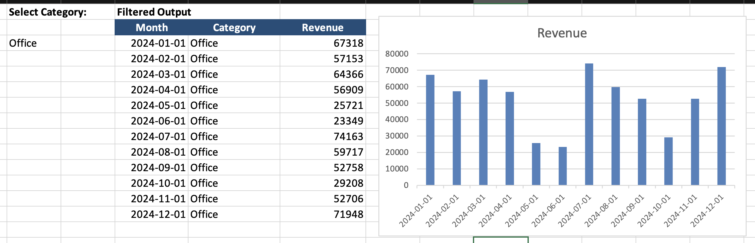
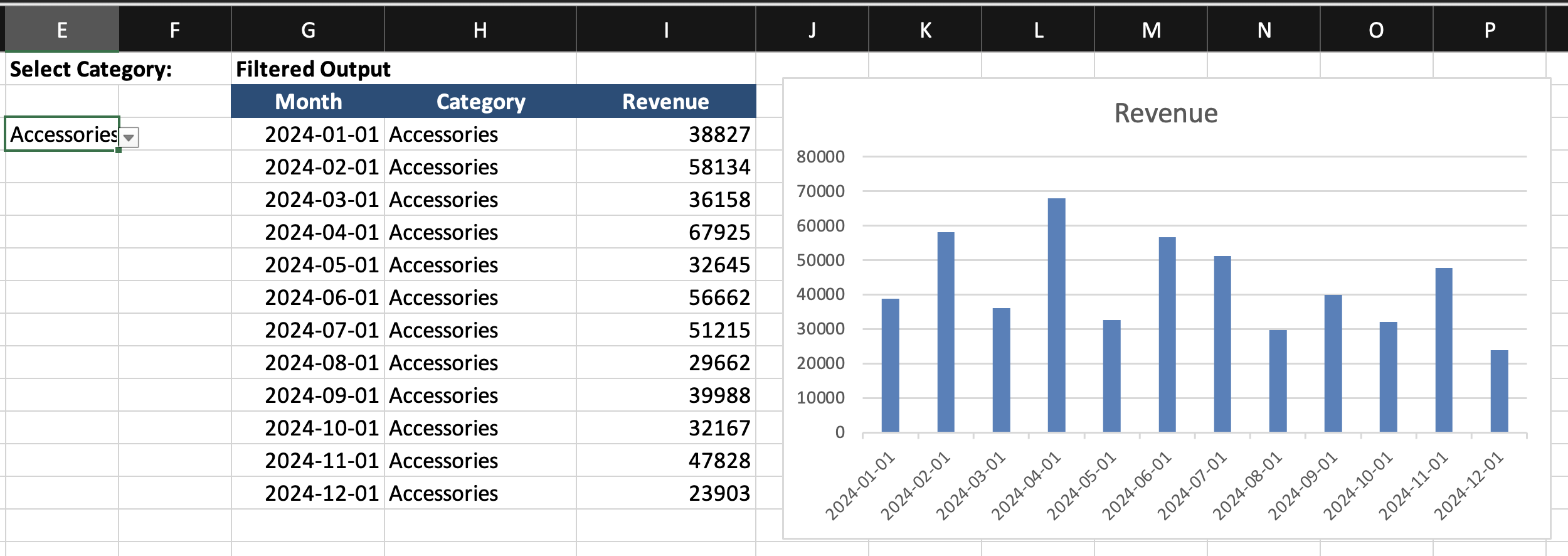
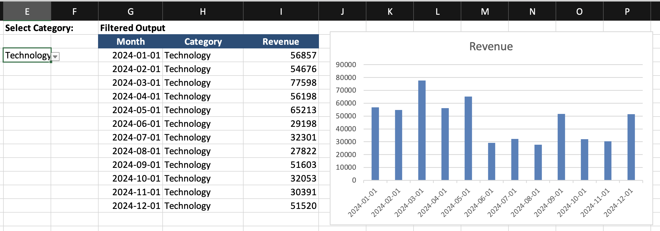
Using the provided dataset:
- Create a dropdown cell to select a Category;
- Use the
FILTERfunction to return matching rows into a separate output area; - Insert a Line or Column Chart based on the filtered output range;
- Change the dropdown selection and confirm that the chart updates automatically.
Goal: build a chart that updates based on a formula-driven data range, not manual filtering.
Thanks for your feedback!
Ask AI

Ask AI

Ask anything or try one of the suggested questions to begin our chat
Dynamic Charts with Formulas
A dynamic chart range is a data range that changes automatically based on a condition or selection. Instead of building a chart from a fixed range, you build it from a formula-driven range. When the formula result changes, the chart updates. The chart itself is not dynamic. The data source is.
How It Works
- A user selects a value from a dropdown;
- A formula returns only the matching rows;
- The chart is built from that formula output;
- When the selection changes, the formula output changes;
- The chart updates automatically.
The key idea: the chart depends on a formula range, not the full dataset.
Creating the Dynamic Range
Assume:
Step 1: Create a Dropdown
- Select an empty cell;
- Go to Data → Data Validation;
- Choose List;
- Select the category range.
Step 2: Create the Formula Output
In a new area, enter: =FILTER(A2:C100; B2:B100=E2)
This creates a dynamic output table.
Step 3: Build the Chart
Insert a chart using the filtered output, not the original data. Now the chart updates when the dropdown changes.
Using the provided dataset:
- Create a dropdown cell to select a Category;
- Use the
FILTERfunction to return matching rows into a separate output area; - Insert a Line or Column Chart based on the filtered output range;
- Change the dropdown selection and confirm that the chart updates automatically.
Goal: build a chart that updates based on a formula-driven data range, not manual filtering.
Thanks for your feedback!
