Summary  
This chapter covers how to define and apply conditional rules to automatically style data elements—based on thresholds, relative rankings, gradients, icon sets, or custom formulas—to highlight patterns and outliers.

General domain of usage  
Data visualization

Conditional formatting in Excel is like giving your data a **visual makeover**. It allows you to automatically apply **specific formatting** to cells that meet certain criteria. 

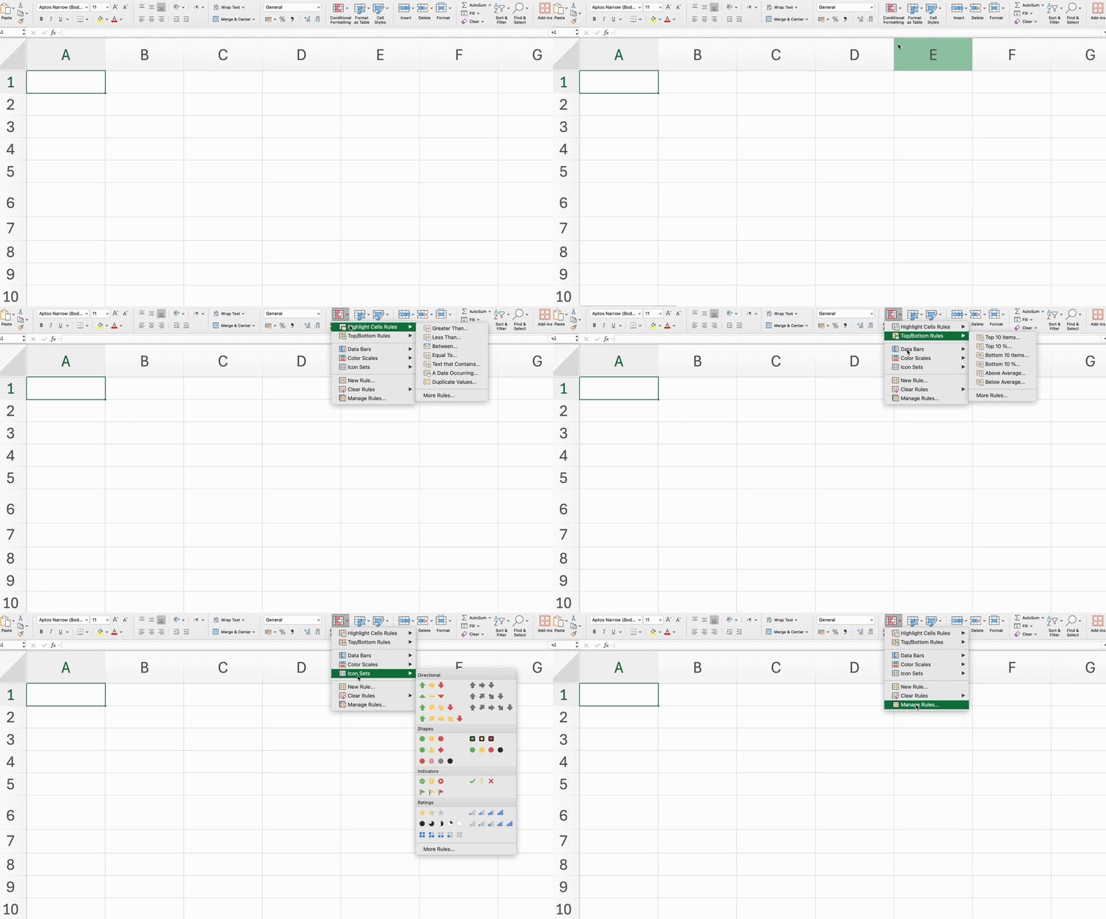
- Apply conditional formatting using the **Highlight Cells Rules** for specific criteria via **Home** tab → **Styles** group;
- Use the **Top/Bottom Rules** to format cells with the **highest** or **lowest** values;
- Add **Data Bars** to visually represent cell values;
- Apply **Color Scales** to show value ranges with a gradient of colors;
- Use **Icon Sets** to represent different values with icons.

Initial Workbook

import unittest
import json
import os


def _dynamic_test(test_case, condition, success_message, failure_message):
    if condition:
        test_case._testMethodName = success_message
        test_case.assertTrue(True, success_message)
    else:
        test_case._testMethodName = failure_message
        test_case.fail(failure_message)


class TestUserCode(unittest.TestCase):
    @classmethod
    def setUpClass(cls):
        cls._no_data = True
        cls.sheet = {}
        cls.styles = {}
        if os.path.exists("payload.json"):
            try:
                with open("payload.json") as f:
                    raw = f.read().strip()
                if not raw:
                    return
                data = json.loads(raw)
            except (json.JSONDecodeError, ValueError):
                return
        else:
            return
        cls._no_data = False
        cls.data = data
        cls.sheet_id = next(iter(data["sheets"]))

        # Parse conditional formatting plugin
        resources = data.get("resources", [])
        cf_resource = next(
            (r for r in resources if r.get("name") == "SHEET_CONDITIONAL_FORMATTING_PLUGIN"),
            {}
        )
        raw = cf_resource.get("data", "{}")
        cf_data = json.loads(raw) if raw else {}
        cls.cf_rules = cf_data.get(cls.sheet_id, [])

    # ------------------------------------------------------------------ #
    # Helpers
    # ------------------------------------------------------------------ #

    def _rules_on_range(self, sr, sc, er, ec):
        """Return all CF rules whose range matches (startRow, startCol, endRow, endCol)."""
        matched = []
        for rule in self.cf_rules:
            for r in rule.get("ranges", []):
                if (r.get("startRow") == sr and r.get("startColumn") == sc
                        and r.get("endRow") == er and r.get("endColumn") == ec):
                    matched.append(rule)
                    break
        return matched

    def _find_rule(self, rules, rule_type, **kwargs):
        """Return first rule dict matching type and optional rule-level kwargs."""
        for entry in rules:
            r = entry.get("rule", {})
            if r.get("type") != rule_type:
                continue
            if all(r.get(k) == v for k, v in kwargs.items()):
                return r
        return None

    # ------------------------------------------------------------------ #
    # Step 1 — Highlight Cells > 90 on C20:F26
    # (0-based rows 19-25, cols 2-5)
    # ------------------------------------------------------------------ #

    def test_highlight_greater_than_90_C20_F26(self):
        if self._no_data:
            _dynamic_test(self, True, "Highlight Cells > 90 applied to C20:F26.", ""); return
        rules = self._rules_on_range(19, 2, 25, 5)
        found = self._find_rule(rules, "highlightCell",
                                subType="number", operator="greaterThan")
        ok = found is not None and found.get("value") == 90
        _dynamic_test(self, ok,
            "Highlight Cells > 90 applied to C20:F26.",
            "Missing: Highlight Cells > 90 on C20:F26. "
            "Select C20:F26 → Conditional Formatting → Highlight Cell → Greater Than → 90.")

    # ------------------------------------------------------------------ #
    # Step 2 — Highlight Cells < 70 on C20:F26
    # ------------------------------------------------------------------ #

    def test_highlight_less_than_70_C20_F26(self):
        if self._no_data:
            _dynamic_test(self, True, "Highlight Cells < 70 applied to C20:F26.", ""); return
        rules = self._rules_on_range(19, 2, 25, 5)
        found = self._find_rule(rules, "highlightCell",
                                subType="number", operator="lessThan")
        ok = found is not None and found.get("value") == 70
        _dynamic_test(self, ok,
            "Highlight Cells < 70 applied to C20:F26.",
            "Missing: Highlight Cells < 70 on C20:F26. "
            "Select C20:F26 → Conditional Formatting → Highlight Cell → Less Than → 70.")

    # ------------------------------------------------------------------ #
    # Step 3 — Bottom 10 Items on B6:E12
    # (0-based rows 5-11, cols 1-4)
    # ------------------------------------------------------------------ #

    def test_bottom_10_B6_E12(self):
        if self._no_data:
            _dynamic_test(self, True, "Bottom 10 Items applied to B6:E12.", ""); return
        rules = self._rules_on_range(5, 1, 11, 4)
        found = self._find_rule(rules, "highlightCell", subType="rank")
        ok = (found is not None
              and found.get("isBottom") is True
              and not found.get("isPercent", False))
        _dynamic_test(self, ok,
            "Bottom 10 Items applied to B6:E12.",
            "Missing: Bottom 10 Items on B6:E12. "
            "Select B6:E12 → Conditional Formatting → Top/Bottom → Bottom → Submit.")

    # ------------------------------------------------------------------ #
    # Step 4 — Data Bar on F6:F12
    # (0-based rows 5-11, col 5)
    # ------------------------------------------------------------------ #

    def test_data_bar_F6_F12(self):
        if self._no_data:
            _dynamic_test(self, True, "Data Bar applied to F6:F12.", ""); return
        rules = self._rules_on_range(5, 5, 11, 5)
        found = self._find_rule(rules, "dataBar")
        _dynamic_test(self, found is not None,
            "Data Bar applied to F6:F12.",
            "Missing: Data Bar on F6:F12. "
            "Select F6:F12 → Conditional Formatting → Data Bar → Submit.")

    # ------------------------------------------------------------------ #
    # Step 5 — Color Scale on C20:F26
    # ------------------------------------------------------------------ #

    def test_color_scale_C20_F26(self):
        if self._no_data:
            _dynamic_test(self, True, "Color Scale applied to C20:F26.", ""); return
        rules = self._rules_on_range(19, 2, 25, 5)
        found = self._find_rule(rules, "colorScale")
        _dynamic_test(self, found is not None,
            "Color Scale applied to C20:F26.",
            "Missing: Color Scale on C20:F26. "
            "Select C20:F26 → Conditional Formatting → Color Scale → Submit.")

    # ------------------------------------------------------------------ #
    # Step 6 — Icon Set on C20:F26 with thresholds 90, 80, 70, 60
    # ------------------------------------------------------------------ #

    def test_icon_set_C20_F26(self):
        if self._no_data:
            _dynamic_test(self, True, "Icon Set applied to C20:F26.", ""); return
        rules = self._rules_on_range(19, 2, 25, 5)
        icon_rules = [entry.get("rule", {}) for entry in rules
                      if entry.get("rule", {}).get("type") == "iconSet"]

        ok = len(icon_rules) > 0
        _dynamic_test(self, ok,
            "Icon Set applied to C20:F26.",
            "Missing: Icon Set on C20:F26. "
            "Select C20:F26 → Conditional Formatting → Icon Set → choose a 3-icon style → Submit.")


if __name__ == "__main__":
    unittest.main()


test_main.py

Dive into the world of Excel with this comprehensive video course, designed to take you from basic navigation to mastering functions and basic data analysis. Starting with foundational skills like data entry and cell formatting, you'll quickly progress to using powerful tools. Whether you're organizing large datasets, performing statistical analysis, or creating dynamic charts, this course equips you with the practical skills needed in today’s data-driven environment.

Kickstart your journey with Excel by understanding its interface, basic functions, and essential data entry techniques. Learn how to navigate toolbars, worksheets, and master the fundamental elements to set a solid foundation.

Dive deeper into Excel by exploring advanced data entry and formatting options. Sharpen your skills in text and number formatting, discover how to effectively use styles, and enhance spreadsheet readability and functionality.

Unleash the power of Excel with an introduction to basic formulas and functions. Gain confidence in creating calculations, using cell references, and employing key functions like SUM, AVERAGE, MIN, and MAX to automate and simplify your data analysis tasks.

In this section, you will master advanced Excel formulas and functions, enhancing your ability to manage complex calculations. Learn to display and audit formulas, utilize nested and logical statements, and apply conditions effectively to streamline your data analysis tasks.

Explore comprehensive techniques for sorting, filtering, and managing data efficiently. This section covers everything from basic data organization to advanced filtering and table management, ensuring you can handle and analyze data effectively.

Dive into the art of data visualization using Excel's powerful charting tools. You'll learn to create various types of charts, customize them to enhance visual appeal, and manipulate data within charts to present clear and compelling visual stories.

Gain proficiency in managing worksheets and workbooks within Excel. This section teaches you how to effectively organize and manipulate workbook elements, utilize formatting tools, and secure your work with passwords, providing a thorough grounding in workbook operations.

Excel Conditional Formatting

Key Points