single
Defining the Number of Clusters
Swipe to show menu
There are several techniques we can use to help us to define the optimal number of clusters. There are also several techniques available for spectral clustering, but they are strongly based on hard math and are not implemented within several functions.
What can we use there? Remember the second section and the silhouette score we considered. We can also use it there.
Let's see what will be the result of building the silhouette scores chart for the circles' data (the scatter plot is below).
12345678910111213141516171819202122232425# Import the libraries import pandas as pd import seaborn as sns import matplotlib.pyplot as plt from sklearn.cluster import SpectralClustering from sklearn.metrics import silhouette_score # Read the data data = pd.read_csv('https://codefinity-content-media.s3.eu-west-1.amazonaws.com/138ab9ad-aa37-4310-873f-0f62abafb038/model_data4.csv', index_col = 0) # Creating lists n_cl = range(2, 10) silhouettes = [] # Calculate the scores for different number of clusters for j in n_cl: model = SpectralClustering(n_clusters = j, affinity = 'nearest_neighbors') model.fit(data) silhouettes.append(silhouette_score(data, model.labels_)) # Visualize the results g = sns.lineplot(x = n_cl, y = silhouettes) g.set_xlabel('Number of clusters') g.set_ylabel('Silhouette score') plt.show()
Swipe to start coding
Build the silhouette score chart for the weather data using silhouette scores and spectral clustering. Follow the next steps:
- Import
SpectralClusteringandsilhouette_scorefunctions fromsklearn.clusterandsklearn.metricsrespectively. - Create a
rangeobject namedn_clwith integer numbers from 2 to 9 (inclusive). - Iterate over
n_cl. On each step:
- Create
SpectralClusteringmodel namedmodelwithjclusters and'nearest_neighbors'affinity. - Fit (
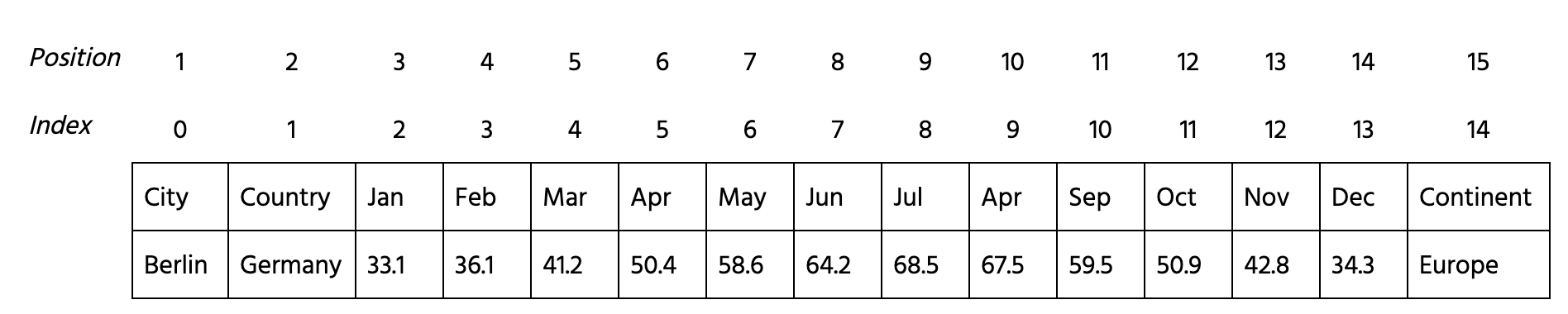
.fit()method) the numerical columns ofdatatomodel. The numerical columns are 3 - 14. - Append to
silhouetteslist the value of silhouette score. Pass the predictedlabels_as the second parameter.
- Build the
seabornline plotn_cl(x-axis) vssilhouettes(y-axis)
Solution
Thanks for your feedback!
single
Ask AI
Ask AI

Ask anything or try one of the suggested questions to begin our chat
